Description
This project aims to produce a model that can forecast the price of Apple Inc. stocks. The S&P500 will be used as an exogenous variable to strengthen model performance. This model can be used on any stock. It can be helpful in our investing strategy as it can provide an indication of what to expect in the future. This helps investors plan ahead to maximize gains and minimize losses.
Objectives
Train a model than can predict the price of the Apple Inc’s stock using ARIMA.
Tools


Python was used for this project. The following libraries were utilized:
- Numpy
- Pandas
- Matplotlib
- seaborn
- scipy
- statsmodels
- Pmdarima
Steps
- Loading packages
- Importing the data from Yahoo!Finance
- Preprocessing the data
- Plotting the data
- Test for Stationarity: ADF test
- Seasonal decomposition
- Differencing
- Log transformation
- KPSS test
- Training the Auto ARIMA model
- Make Predictions
- Evaluate Model Performance
The Data
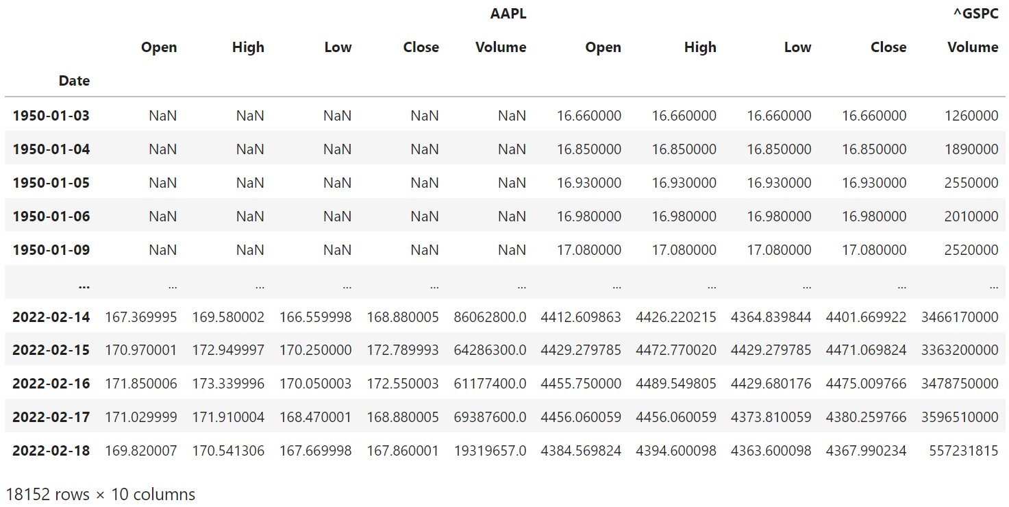
The stock data for Apple Inc. (APPL) and the S&P500 (^GSPC) were taken directly from Yahoo! Finance using the yfinance library.
raw_data = yfinance.download(tickers= "AAPL, ^GSPC", interval="1d",auto_adjust = True, treads=True, group_by='ticker')
Plotting the Data
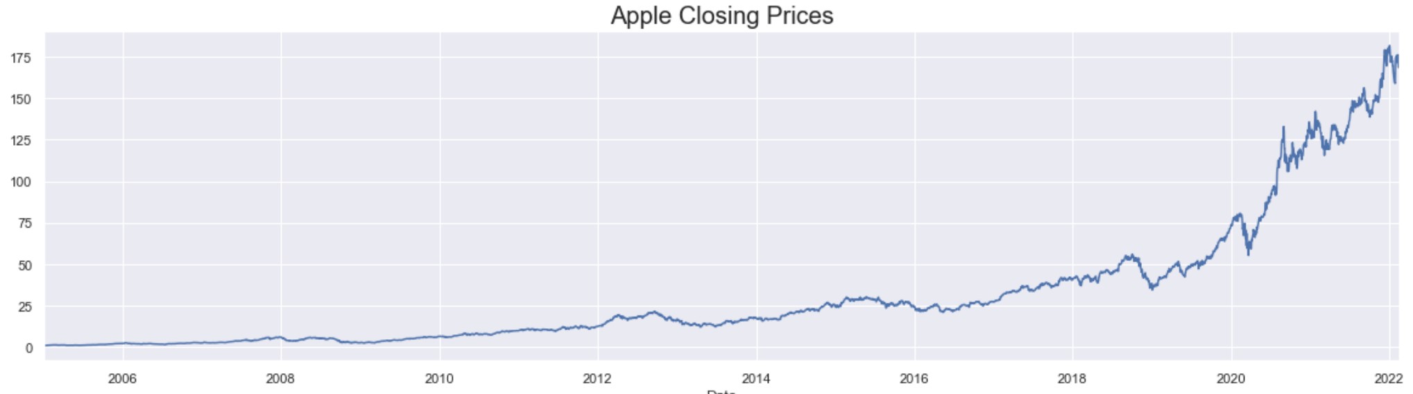
The graph shows that there has been an exponential increase in the stock price of Apple in the last 4 years.
When we take each year separately as in the graph below, we can see that there is an increasing trend especially in the more recent years.
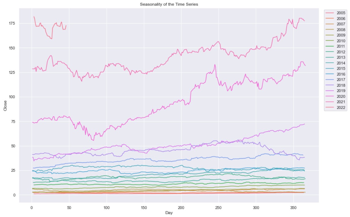
The graph shows that in the first half of the time series data (2005-2015) the stock price was below $25 with very small movement in the price. The latter years in the dataset show that the price had greater movements and continuosly increased breaching $175. 2019-2021 showed a steeper upward trend compared to previous years.
Test for Stationarity: ADF test
The Augmented Dickey Fuller test is a way to check the stationarity of a timeseries.
Null hypothesis : The data is non-stationary
Alternative Hhypothesis : The data is stationary
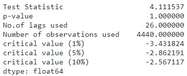
The ADFuller test shows a p-value of 1 which is significantly greater than the significance level of 0.05. The test statistics is also greater than the critical values. This means that the time series data is non-stationary. Since the data is non-stationary, we will use the ARIMA model since it is best suited for this type of data.
Seasonal Decomposition
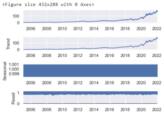
The figure above shows that there is no seasonality in the price of Apple stocks.
Differencing
Differencing is a method of transforming a non-stationary time series into a stationary one where the values are the differences between consecutive values of the original data.
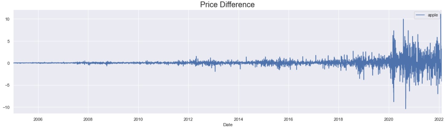
The graph above shows that differencing still produced a data that is non-stationary. The variance towards the end of the data set is much larger than in the earlier years.
Log Transformation
Log transformation is a data transformation method in which each variable x is replaced with a log(x). Log transformation was performed on the differenced data. The graph of the log transformed data is presented below.
![]()
![]()
The AD fuller test shows a p-value of less that 0.05 and the test statistic is less than the critical value. This confirms that the data is now stationary. The graph shows that the variace is more constant aside from huge spikes in late 2008 and early 2020. These huge spikes pertain to the 2008 financial crisis and the start of the COVID-19 pandemic, respectively.
KPSS Test
The KPSS test is another way to determine if a time series data is stationary or not. The null and alternative hypothesis of this test are the opposite that of the ADF test.
Null hypothesis : The data is stationary
Alternative Hhypothesis : The data is non-stationary
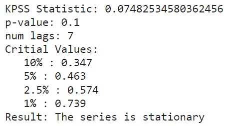
The KPSS confirms the findings of the ADF test that our timeseries data after differencing and log transformation is stationary.
Auto ARIMA Model
The model was trained using auto ARIMA with. The data was split with 90% used for training and the remaining 10% used for testing. The resulting model is a SARIMAX model (1,0,1)x(3,1,1,12). Below is the diagnostics of the model.
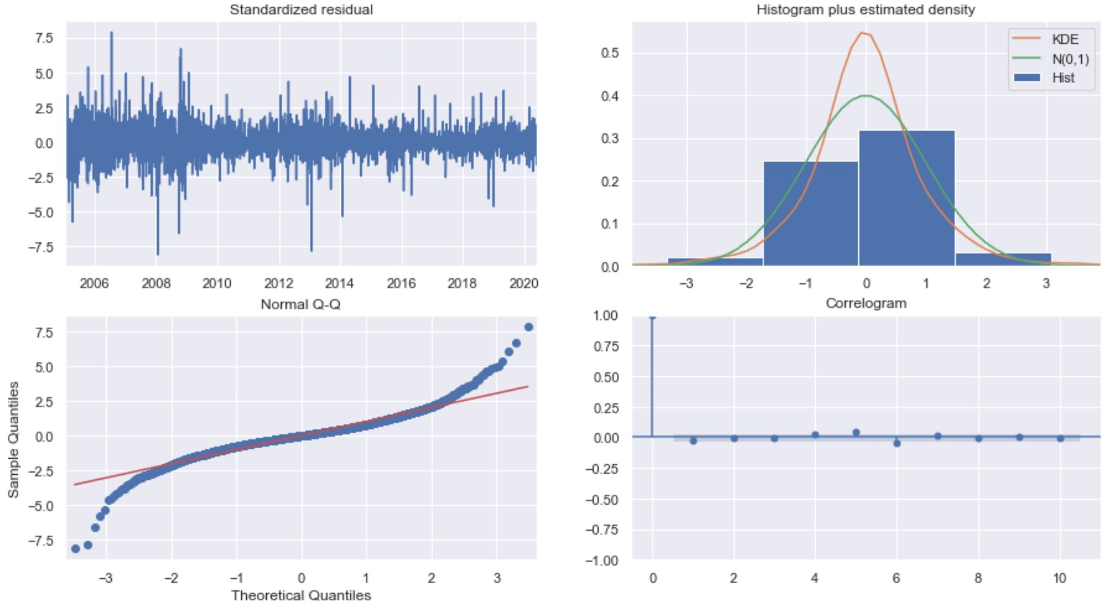
Top left: The residual errors fluctuate around the mean of 0 and have a uniform variance.
Top right: The density plot suggest the residuals have a normal distribution with a mean of zero.
Bottom left: The QQ plot also show that the residuals have a normal distribution.
Bottom right: The ACF plot shows that the residual errors are not autocorrelated.
Make Predictions & Evaluate Model Performance
Using the trained model, we predicted the stock price of Apple for the remaining 10% of the dates included in the dataset. We then compared these predicted prices with the actual prices on those dates. The graph below summarizes the performance of the model when compared to the actual values.
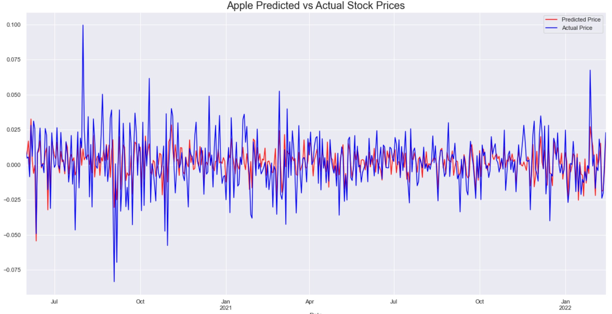
We can see that the predictions came very close to the actual values.
The model has an RMSE of 14.011 which means that its predictions will have a little difference with the actual prices and this difference will have a mean of $14.
The project can be accessed on GitHub through this link.